
This is the official NCERT Class 10 Mathematics Chapter 14 — Probability, which runs from page 201 to page 217 in the printed book. If you came looking for the probability class 10 chapter 14 PDF, the official file from ncert.nic.in is linked right below.
This page is maintained for the current academic session; under the download you will find what the chapter contains, its key ideas and the mistakes to avoid.
Download the Official Chapter 14 PDF
The official Probability Class 10 NCERT Chapter 14 PDF from ncert.nic.in opens the complete textbook chapter, pages 201 to 217 — the theory, its worked examples, every question of Exercise 14.1, the summary and the closing note to the reader.
It is the official edition published by NCERT and opens in any browser without a login.
Chapter 14 at a Glance
Before you open the PDF, here is the shape of what is inside — and what makes this chapter different from the ones around it.
The table on this page lists how much the chapter holds — its sections, figures, worked examples and exercise questions — so you know at a glance how long the file is.
The chapter opens with a short epigraph and a history note, then builds the theoretical definition of probability through worked examples that ask repeated “(Why?)” prompts — each one a check that you know where the counts came from. Exercise 14.1 is the chapter’s single exercise; section 14.2 is the summary; and a closing “Note to the reader” links empirical and theoretical probability.
Two things stand out inside: the 6 by 6 two-dice grid in Example 13 (the 36 ordered pairs), and the partially filled sum table in Question 22, which is the same grid viewed from the side of the total. The chapter runs from NCERT page 201 to page 217.
What This Chapter Covers
This tour follows the chapter’s argument in order, so you can read it as a map before you open the PDF.
Why the chapter exists. In Class 9 you met empirical probability from repeated trials. That works only when an experiment can be repeated many times; it fails for one-off events such as a satellite launch failing or an earthquake destroying a building, which nobody repeats for practice (NCERT, p. 203). The chapter replaces repetition with an assumption.
The assumption. Outcomes are equally likely. A fair coin has no reason to favour a side; a bag with 4 red balls and 1 blue ball makes “red” and “blue” unequal chances, so the colours are not equally likely even though the individual balls are (NCERT, p. 203). From here on the chapter assumes equal likelihood and builds on it.
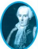
Where the idea came from. Laplace gave the definition in 1795. The theory began in the 16th century with J. Cardan’s Book on Games of Chance; later work came from James Bernoulli (1654-1705), A. de Moivre (1667-1754) and Laplace’s Theorie Analytique des Probabilites of 1812 (NCERT, p. 204).
The examples then move from the simplest cases to the counting frameworks you will reuse in every question:
| Example | Experiment | Idea it teaches |
|---|---|---|
| 1 | tossing a coin once | the definition applied to the simplest case, with both outcomes equal |
| 2 | drawing one ball from a bag of three differently coloured balls | equal likelihood across outcomes |
| 3 | throwing a die once | complementary parts of the same experiment |
| 4 | drawing one card from a shuffled deck | the deck structure and the complement rule |
| 5 | a tennis match between two players | complementary events |
| 6 | two friends’ birthdays | the complement trick for “same” versus “different” |
| 7 | selecting a class representative | counting a named subgroup (girls, boys) |
| 8 | drawing a marble from a mixed box | totalling the bag before counting favourable outcomes |
| 9 | tossing two different coins | ordered outcomes: four, not three |
| 12 | a carton of good and defective shirts | deciding what “favourable” means for each trader |
| 13 | two dice thrown together | the 36-outcome grid and its sums |
The two starred examples break the pattern: Example 10 uses a length on a number line and Example 11 uses an area, because here the outcomes are infinitely many (NCERT, pp. 210-212). The chapter then returns to counting with Example 12 (shirts) and Example 13 (two dice), closes with Exercise 14.1, the six-point summary and the note to the reader (NCERT, pp. 214-217).
Key Concepts: The Ideas That Run the Chapter
This chapter measures how likely an event is on a scale from 0 to 1 by counting outcomes — that is why NCERT calls it theoretical rather than empirical. These are the ideas you use in every question.
- The definition and its two requirements. \( P(E) = \frac{\text{Number of outcomes favourable to } E}{\text{Number of all possible outcomes}} \) works only when the outcomes are equally likely and the set of outcomes is finite. If either fails, the formula does not apply (NCERT, p. 203).
- Checking “equally likely”. A red ball and a blue ball drawn from a bag of 4 red and 1 blue are not equally likely, because red has four chances and blue has one. Draw by colour: unequal. Draw by individual ball: equal (NCERT, p. 203).
- Elementary events add to 1. An event with exactly one outcome is elementary; the probabilities of all elementary events of an experiment sum to 1 (NCERT, p. 205).
- The complement. Write “not E” as \( \bar{E} \). Then \( P(\bar{E}) = 1 – P(E) \) (NCERT, p. 206).
- The boundaries. An impossible event has probability 0; a sure event has 1; everything lies in between, so \( 0 \leq P(E) \leq 1 \) (NCERT, p. 207).
- The counting frameworks. A coin has 2 outcomes; a die has 6; two dice have 36 ordered pairs; a deck has 52 cards in 4 suits of 13, with kings, queens and jacks as face cards; a bag’s total is just the count of items inside (NCERT, pp. 204-213).
- Geometric probability (starred). When outcomes are all points of a line or a region, the count formula fails; probability becomes a ratio of lengths or areas (NCERT, pp. 210-212).
Worked Example: The Complement Rule With New Numbers
NCERT’s examples use the book’s own values; this one uses fresh numbers so you can practise the same move. In a class of 60 students, 18 wear spectacles. What is the probability that a randomly chosen student does not wear spectacles?
Step 1: Let E be “the student wears spectacles”.
There are 60 equally likely students, and 18 are favourable to E.
\[ P(E) = \frac{18}{60} = \frac{3}{10} \]
Step 2: “Not spectacles” is the complement \( \bar{E} \), so subtract from 1.
\[ P(\bar{E}) = 1 – P(E) = 1 – \frac{3}{10} = \frac{7}{10} \]
Final answer: \( P(\text{not spectacles}) = \frac{7}{10} \).
Key Formulas: What to Memorise and What Each Part Means
These are the only formulas this chapter builds on; every exercise is one of these applied to a new situation. Learn what each symbol means, not just the shape of the formula.
| Formula | What each symbol means | Where it appears |
|---|---|---|
| \( P(E) = \frac{\text{Number of outcomes favourable to } E}{\text{Number of all possible outcomes}} \) | \(E\) is the event; the outcomes must be equally likely | NCERT p. 203, the definition |
| \( P(E_1) + P(E_2) + \dots + P(E_n) = 1 \) | \(E_1, E_2, \dots, E_n\) are the elementary (single-outcome) events | NCERT p. 205 |
| \( P(\bar{E}) = 1 – P(E) \) | \( \bar{E} \) is “not E”, the complement of the event | NCERT p. 206 |
| \( 0 \leq P(E) \leq 1 \) | impossible event = 0; sure event = 1; nothing outside | NCERT p. 207 |
| \( P(E) = \frac{\text{favourable length or area}}{\text{total length or area}} \) | used when outcomes are all points of a line or region | NCERT p. 211 (starred) |
Use row 1 whenever you can count outcomes. Reach for row 3 whenever the question says “not”, “does not”, “at least” or “without”. Row 5 belongs only to the starred geometric examples.
Definitions You Must Know
These are the chapter’s exact terms in student language, each tied to the page where NCERT introduces it. Batch them while revising — the exam reuses this vocabulary.
| Term | Meaning in one line | NCERT page |
|---|---|---|
| Theoretical (classical) probability | favourable outcomes divided by all possible outcomes, assuming equal likelihood | p. 203 |
| Equally likely outcomes | each outcome has the same chance as every other | p. 203 |
| Empirical probability | trials in which the event happened, divided by total trials — from observation, not assumptions | p. 203 |
| Elementary event | an event with exactly one outcome | p. 205 |
| Complementary events | \(E\) and \( \bar{E} \); “not E”, with probabilities adding to 1 | p. 206 |
| Impossible event | cannot happen; probability 0 | p. 207 |
| Sure (certain) event | must happen; probability 1 | p. 207 |
| Fair (unbiased) coin, random toss | a symmetrical coin with no side favoured, tossed without interference | p. 203 |
| Face cards | kings, queens and jacks in a deck | p. 207 |
Reading the Chapter’s Figures

Each of the chapter’s figures carries a different kind of idea — history, length, area and a practice question. Here is what each one shows and how NCERT uses it.
The Historical Portrait: Where Probability Began
This portrait opens the chapter’s history note (NCERT, p. 204). The text around it tells the story: Cardan wrote about games of chance in the 16th century; James Bernoulli (1654-1705) and A. de Moivre (1667-1754) advanced the subject; and Laplace’s Theorie Analytique des Probabilites (1812) is described as the greatest contribution by a single person to probability theory.
Probability is now used in biology, economics, genetics, physics and sociology.
Fig 14.1: Probability as a Length (Example 10)
In the musical chair game, the music can stop at any instant between 0 and 2 minutes, so the outcomes are all points of a length — not countable. The favourable part is the first half-minute, a length of \( \frac{1}{2} \) out of a total of 2. NCERT computes the probability as the ratio of lengths:
\[ P(E) = \frac{\text{favourable distance}}{\text{total distance}} = \frac{\frac{1}{2}}{2} = \frac{1}{4} \]
This example carries an asterisk — NCERT marks it as not from the examination point of view (NCERT, p. 210).
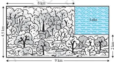
Fig 14.2: Probability as an Area (Example 11)
The helicopter is equally likely to crash anywhere in the rectangle, so the favourable “outcomes” are the lake’s area out of the whole region’s area. The whole region is \(4.5 \times 9 = 40.5\ \text{km}^2\) and the lake is \(2.5 \times 3 = 7.5\ \text{km}^2\), giving \[ P(\text{crash in the lake}) = \frac{7.5}{40.5} = \frac{75}{405} = \frac{5}{27} \]
This is the chapter’s cleanest example of probability as a ratio of areas, and it is also starred as not from the examination point of view (NCERT, p. 211).
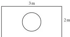
Fig 14.6: A Die Dropped on a Rectangle (Question 20)
This is the practice version of the same area idea. The die is equally likely to land anywhere on the rectangle, so the probability is a ratio of areas:
\[ P(\text{lands inside the circle}) = \frac{\text{area of the circle}}{\text{area of the rectangle}} \]
The circle has diameter 1 m, so its radius is 0.5 m and its area is \( \pi(0.5)^2 = \frac{\pi}{4}\ \text{m}^2 \). The rectangle’s dimensions are labelled on the figure itself — read them off, multiply for the rectangle’s area, and divide. NCERT stars this question too (NCERT, p. 216).
Common Mistakes Students Make in This Chapter
Most lost marks here come from counting outcomes wrongly, not from the formula. NCERT’s own questions are built to catch these six traps, so meet them before the exam does.
| Mistake | Correct rule | How to check your answer |
|---|---|---|
| Assuming outcomes are equally likely when they are not (Question 2: a car starts or does not start; a basketball shot goes in or misses) | Equally likely means each outcome has the same chance; a car usually starts, and a skilled shot usually goes in. By contrast, a true-false answer being right or wrong has two symmetric outcomes and is equally likely (NCERT, p. 214) | Ask: “Is there any reason one outcome should appear more often?” If yes, the count formula does not apply |
| Counting two coins as three outcomes — HH, TT, “one of each” — with probability \( \frac{1}{3} \) each (Question 25(i)) | The outcomes are HH, HT, TH, TT: head-tail and tail-head are different because the coins are distinct (or first and second). Each has probability \( \frac{1}{4} \) (NCERT, pp. 210, 217) | Name the coins (coin A, coin B) and list ordered pairs |
| Giving every two-dice sum from 2 to 12 a probability of \( \frac{1}{11} \) (Question 22(ii)) | The 36 ordered pairs are equally likely; sums have different counts, so their probabilities differ | Count how many pairs give each sum; the counts must total 36 |
| Writing a probability outside 0 to 1, such as -1.5 (Question 4) | \( 0 \leq P(E) \leq 1 \); a negative answer or one above 1 is impossible | If your answer is negative or greater than 1, recount |
| Forgetting that taking an item out changes the total (Question 15(ii): the queen is put aside, so only 4 cards remain; Question 17(ii): the drawn bulb is not replaced, so 20 becomes 19) | “Without replacement” shrinks the denominator by 1 and removes that item from the favourable count | Re-read the question for “put aside” or “not replaced” and adjust the total before the second draw |
| Confusing empirical and theoretical probability | Empirical comes from trials that actually happened; theoretical comes from the equally-likely assumption; the two draw closer as trials increase | Check which definition the question is asking for (NCERT, p. 217) |
Exam Notes: How to Practise This Chapter
Here is where to spend your revision time, using the markers NCERT itself puts in the text. No promises about questions — just an honest map of the material.
- Know which parts NCERT marks as extras. Example 10, Example 11 and Question 20 carry an asterisk with the note “not from the examination point of view” (NCERT, pp. 210, 211, 216). The other examples and all other questions are your core practice.
- Match questions to ideas. The table below maps Exercise 14.1 to the skill each question checks.
| Questions | Idea they test |
|---|---|
| Q1 | the vocabulary: complement, impossible, sure, elementary events, the 0 to 1 bound |
| Q2, Q25 | whether two possible outcomes are actually equally likely, not just both possible |
| Q5, Q7, Q8(ii) | the complement rule \( P(\bar{E}) = 1 – P(E) \) |
| Q13, Q14, Q18 | straight counting of favourable outcomes (die, cards, numbered discs) |
| Q22, Q24 | two-dice problems and the 36-outcome grid |
| Q15(ii), Q17(ii) | removing an item without replacement changes the total |
| Q12, Q21 | everyday decisions — what “favourable” means in a practical context |
- Treat the “(Why?)” prompts as self-checks. Each one asks for the total number of outcomes or the equally-likely assumption behind the previous step. If you can answer them aloud, you understand the counting.
- What a full-marks answer includes. Name the event, state the total number of equally likely outcomes, state the favourable count, and write the probability as a reduced fraction — showing each of the book’s “(Why?)” steps on the way.
- A reading order. Start with the definition formula, then the complement rule, then the 0 to 1 boundaries; after that, do one problem of each type listed above. Leave the starred geometric examples (length and area) for after everything else.
- Syllabus note. Textbook contents and the examinable syllabus are not always identical — check the current official syllabus before deciding what to revise.
The Six Points to Remember From This Chapter
The chapter ends with its own six-point summary (NCERT, p. 217). This is the fastest possible revision for the whole topic.
- The theoretical (classical) probability of an event E is \( \frac{\text{outcomes favourable to E}}{\text{all possible outcomes}} \), assuming the outcomes are equally likely.
- The probability of a sure (certain) event is 1.
- The probability of an impossible event is 0.
- For any event E, \( 0 \leq P(E) \leq 1 \).
- An elementary event has exactly one outcome, and the probabilities of all elementary events of an experiment sum to 1.
- For any event E, \( P(E) + P(\bar{E}) = 1 \); E and \( \bar{E} \) are complementary events.
The closing note adds the link between the two probabilities: empirical probability records what has happened in past trials, while theoretical probability predicts on the basis of assumptions; as the number of trials grows, the empirical value approaches the theoretical one (NCERT, p. 217).
A quick memory aid: “zero for impossible, one for sure, everything between — and the complement always brings you back to one.”
Related Resources
This listing is maintained for the 2026-27 academic session using the NCERT textbook information available to us. NCERT remains the authority for confirming the latest edition.
If you are revising this chapter as part of a larger plan, these pages on this site will take you further.
- Class 10 Mathematics notes — every chapter of the book in revision form.
- Statistics (Chapter 13) — the previous chapter, on mean, median and mode.
- Class 10 study hub — all subjects in one place.
- CBSE notes home — explore by class and subject.
You can also verify the current edition of the book on the official NCERT textbook index at ncert.nic.in/textbook.php.
Sources and Data Verification
Plain facts about what this page describes, and which authority settles what.
- The figures, page numbers and content on this page describe the NCERT Class 10 Mathematics textbook, Chapter 14 (Probability), English edition, NCERT pages 201 to 217, official PDF on ncert.nic.in.
- This page covers only this chapter of this book. It does not cover other chapters or the NCERT Exemplar problem sets.
- The listing is maintained from the NCERT information available to us. NCERT settles textbook editions, chapters and PDFs; CBSE settles curriculum, syllabus and examinations.
| What the chapter holds | Count | Where it is used |
|---|---|---|
| Printed pages | 16 | |
| Sections in the chapter | 2 | |
| Figures with NCERT captions | 4 | |
| Tables | 2 | |
| Exercise questions | 24 | answered in our NCERT Solutions |
| Official NCERT PDF | Download the chapter PDF | the chapter exactly as NCERT publishes it |
Frequently Asked Questions
Answers to the long-tail questions students actually search about this chapter, each grounded in the textbook.
What is the formula for probability in Class 10, and what does each part of it mean?
The formula is \( P(E) = \frac{\text{Number of outcomes favourable to } E}{\text{Number of all possible outcomes}} \). \(E\) is the event you are measuring; the numerator counts outcomes that make E happen; the denominator counts every outcome the experiment can produce; and the whole formula assumes the outcomes are equally likely (NCERT, p. 203).
When a die is thrown, for instance, the denominator is 6 because the die has six equally likely faces.
Why are “the car starts or does not start” outcomes not equally likely?
Two outcomes existing does not make them equally likely. A car usually starts, so “starts” happens far more often than “does not start”; the two outcomes do not have equal chances (NCERT, p. 214, Question 2). Contrast this with a true-false question: a guessed answer being right or wrong has two symmetric outcomes, so those are equally likely.
Always ask whether the experiment is fair before applying the formula.
When two coins are tossed together, why are there four outcomes and not three?
Because the coins are distinct — NCERT’s Example 9 tosses a one-rupee coin and a two-rupee coin together — so “head on the first, tail on the second” is a different outcome from “tail on the first, head on the second” (NCERT, p. 210). The four equally likely outcomes are HH, HT, TH and TT.
The event “one of each” therefore contains HT and TH — two outcomes — so its probability is \( \frac{2}{4} = \frac{1}{2} \), not \( \frac{1}{3} \).
When two dice are thrown, why are there 36 outcomes, and what is the probability of each sum from 2 to 12?
The first die can show any of 6 numbers, and each pairs with any of the 6 numbers on the second die, giving \( 6 \times 6 = 36 \) ordered pairs; NCERT notes that (1, 4) is different from (4, 1) (NCERT, p. 213). The sums are not equally likely because different sums come from different numbers of pairs.
For example, sum 5 comes from the four pairs (1,4), (2,3), (3,2) and (4,1), so its probability is \( \frac{4}{36} = \frac{1}{9} \). The full table is:
| Sum | 2 | 3 | 4 | 5 | 6 | 7 | 8 | 9 | 10 | 11 | 12 |
|---|---|---|---|---|---|---|---|---|---|---|---|
| Probability | \( \frac{1}{36} \) | \( \frac{1}{18} \) | \( \frac{1}{12} \) | \( \frac{1}{9} \) | \( \frac{5}{36} \) | \( \frac{1}{6} \) | \( \frac{5}{36} \) | \( \frac{1}{9} \) | \( \frac{1}{12} \) | \( \frac{1}{18} \) | \( \frac{1}{36} \) |
Each fraction is the count of pairs giving that sum, over 36. These probabilities add to 1, which is your built-in check — and this is exactly the table Question 22 asks you to complete (NCERT, p. 215).
Which of these cannot be the probability of an event: 2/3, -1.5, 15%, 0.7?
-1.5 cannot be a probability, because every probability lies between 0 and 1 inclusive (NCERT, p. 207). The other three are all in range: \( \frac{2}{3} \), 15% (that is, 0.15), and 0.7. If your working ever produces a probability below 0 or above 1, you have counted the wrong way.
How do you find the probability that a dropped die lands inside a circle drawn on a rectangle?
The die is equally likely to land anywhere on the rectangle, so the answer is a ratio of areas (NCERT, p. 216, Question 20). Take the circle’s area as the favourable part and the rectangle’s area as the total: \( P = \frac{\text{area of circle}}{\text{area of rectangle}} \).
The circle has diameter 1 m, hence radius 0.5 m and area \( \pi(0.5)^2 = \frac{\pi}{4}\ \text{m}^2 \). Read the rectangle’s length and breadth from the figure, multiply them, and divide \( \frac{\pi}{4} \) by that product. The question is starred as not from the examination point of view, but the method is the same area idea as Example 11.
Reference: NCERT Class 10 Mathematics textbook, chapter 14, official edition on ncert.nic.in.
Explore Class 10 Mathematics Books
Related chapters: