
Introduction to Graphs Class 8 is chapter 13 of the NCERT Class 8 Mathematics textbook — the chapter that turns tables of numbers into pictures you can read at a glance. The official 14-page PDF is right here, followed by a plain-language walkthrough of its sections, five key figures and both exercises.
Download the Introduction to Graphs Class 8 Chapter PDF
The Introduction to Graphs Class 8 NCERT chapter PDF is published by NCERT on ncert.nic.in and runs to 14 printed pages. Open it for the full chapter text — Section 13.1 on line graphs, Section 13.2 on applications, all the worked examples, the figures and Exercises 13.1 and 13.2 — exactly as it appears in the printed book.
The file belongs to the current NCERT Class 8 Mathematics textbook, whose other chapters are also on the official NCERT site.
Chapter 13 at a Glance
The table below lists what the Chapter 13 file holds, in one place.
| Item | Count |
|---|---|
| Main sections | 3 |
| Figures explained on this page | 5 |
| Worked examples | 4 |
| Exercise questions | 8 |
If you are reading this chapter for the first time, start at Section 13.1. If you are revising, jump to the exercise mapping and the common-mistakes table below.
What This Chapter Covers: From Temperature Records to Petrol Costs
This chapter builds one skill in two stages: first you learn to read a graph that is already drawn, then you learn to draw a graph from a table of values. Each stage ends with an exercise so you can check yourself as you go.
| Stage | What you learn | Example that teaches it | How you practise |
|---|---|---|---|
| 13.1 Introduction and a line graph | Reading line graphs: axes, points, coordinates, trends | Renu’s time-temperature record; Example 1 (two batsmen over ten matches); Example 2 (a car’s journey from city P to city Q, 350 km apart) | Exercise 13.1 |
| 13.2 Some Applications | Independent and dependent variables, direct variation, drawing linear graphs | Petrol quantity and cost; simple interest on deposits; Ajit’s scooter at a constant speed of 30 km per hour | Exercise 13.2 |
Example 1 asks you to compare two batsmen’s scores and judge who is the steadier; Example 2 follows a car hour by hour and asks when it stopped and when it reached city Q. Both teach the reading skill that Exercise 13.1 then tests.
Key Concepts You Need Before the Exercises
These five ideas appear in almost every question in the chapter. Each one below comes with a reason and a named example from the book.
- Axes. The horizontal line is the x-axis and the vertical line is the y-axis. In Renu’s graph the x-axis carries time and the y-axis carries temperature, and each axis is labelled with the quantity it shows.
- Coordinates. Every row of a table becomes one plotted point. The petrol table gives the points (10, 500), (15, 750), (20, 1000) and (25, 1250), one point per row.
- Scale. Equal divisions on an axis represent fixed amounts — Example 4 uses 1 unit = ₹100 on the deposit axis and 1 unit = ₹10 on the interest axis. The scale is chosen so that every point fits on the sheet and in-between values can still be read.
- Line graph vs linear graph. A line graph is made by joining points with line segments; it is linear only when all the plotted points lie on one straight line. Renu’s temperature graph is a line graph but not a linear graph. The side-of-square graphs in Exercise 13.2 compare linear and non-linear graphs in one go: perimeter against side is linear, area against side is not.
- Dependent and independent variables. The quantity you choose or control is the independent variable; the quantity that responds to it is the dependent variable. Electricity used is independent, and the electricity bill is dependent.
Definitions From the Chapter, in Plain Words
These are the terms a teacher will expect you to use correctly in an answer, wherever the chapter introduces them.
| Term | Plain meaning | Where it appears |
|---|---|---|
| Line graph | Data that changes continuously over time, shown by points joined with line segments. | Section 13.1.1, Renu’s temperature record |
| Linear graph | A line graph in which all the plotted points lie on one unbroken straight line. | Example 3 (petrol cost) and Example 5 (time-distance) |
| x-axis | The horizontal line on the graph; usually carries the independent quantity such as time or number of litres. | Section 13.1.1 |
| y-axis | The vertical line; usually carries the quantity being measured, such as temperature or cost. | Section 13.1.1 |
| Independent variable (or control variable) | The quantity you choose or control; plotted on the x-axis. | Section 13.2, electricity used |
| Dependent variable | The quantity that responds to the independent one; plotted on the y-axis. | Section 13.2, electricity bill |
| Coordinates | The pair (x-coordinate, y-coordinate) that fixes one point on the graph sheet. | Closing summary, “What Have We Discussed” |
Reading the Chapter’s Figures, Step by Step
Each figure below is one idea made visible. For every one, look at the axes first, then the points, then the line — the order never changes. You will meet the same graphs again in the exercises.
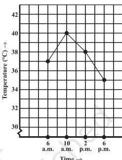
This is Renu’s temperature record before the points are joined. The first thing to notice is that each reading — the time and the temperature together — becomes one point, not two separate values.
That is the whole logic of a graph: a row in a table becomes a mark on the grid, and the position of that mark answers “how much, at what time”.
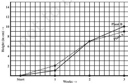
This graph belongs to Exercise 13.1 Question 3. Two plants share one set of axes, so you can compare their growth without reading the table at all. To answer, find the week on the x-axis, move up to the correct plant’s line, then across to the height on the y-axis.
Question 3(g) asks whether the plants were ever the same height in the weeks shown — check whether the two lines share a point at any recorded week.

This figure opens Section 13.2, and it is the chapter’s clearest example of the two variables: the electricity you use is chosen by you (independent), and the bill responds to it (dependent). The independent quantity goes on the horizontal axis and the dependent one on the vertical axis — the rule the chapter applies in every graph it draws.
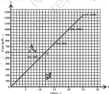
This is the graph of Example 3, where 10 litres cost ₹500 and 15 litres cost ₹750. Look at two things. First, the points (10, 500), (15, 750), (20, 1000) and (25, 1250) all lie on one straight line, so this is a linear graph. Second, that straight line passes through the origin — 0 litres cost ₹0 — which is the signature of direct variation: double the litres, and the cost doubles.

This figure demonstrates the reading method you will use all chapter. To find the cost of 12 litres: locate 12 on the horizontal axis, go vertically up until you meet the graph, then horizontally across to the vertical axis — the meeting point is the cost.
Reading backwards means starting from the value you already know on one axis, tracing across to the line, then down to the other axis. That is how the Try These question finds what ₹800 buys — at ₹50 per litre, \(800 \div 50 = 16\) litres — and how Example 4 finds the deposit needed to earn ₹70 interest.
Worked Example With New Numbers: A Bus Journey
This original example runs the plotting routine — the “Steps to follow” list inside Example 4 — on a fresh set of numbers, so you can copy the routine in an exam. A bus leaves its stop at 8 a.m., and its distance from the stop is noted every hour.
| Time | 8 a.m. | 9 a.m. | 10 a.m. | 11 a.m. | 12 noon |
|---|---|---|---|---|---|
| Distance from stop (in km) | 0 | 25 | 50 | 50 | 80 |
Step 1 — Identify the quantities: time of day and distance from the stop.
Time is the independent quantity; distance responds to it.
Step 2 — Decide the axes: time on the horizontal (x) axis and distance on the vertical (y) axis.
This matches every graph in the chapter: independent on the x-axis, dependent on the y-axis.
Step 3 — Choose a scale: horizontal, 1 unit = 1 hour (the five readings span 8 a.m. to 12 noon); vertical, 1 unit = 10 km (the distances run from 0 to 80 km).
The scale exists so that all points fit on the sheet and in-between values can still be read.
Step 4 — Plot the points: \((8, 0)\), \((9, 25)\), \((10, 50)\), \((11, 50)\), \((12, 80)\).
Step 5 — Join the points: the segments now tell a story — steady travel, a stop, then faster travel.
Now read from the graph the way Exercise 13.1 asks you to.
- Distance at 10:30 a.m.: 10:30 lies halfway between 10 a.m. and 11 a.m. on the x-axis, and the graph above it is the flat segment at 50 km. The bus is 50 km from the stop at 10:30.
- The flat segment from 10 to 11 a.m.: time is passing while the distance stays at 50 km. A horizontal segment on a time-distance graph means the vehicle has stopped — not that it moved at a steady speed. This is exactly the reasoning Example 2 uses when the car stays at 200 km from 11 a.m. to 12 noon.
- Distance at 11:30 a.m.: 11:30 is halfway along the segment from \((11, 50)\) to \((12, 80)\). The distance rises by 30 km over that hour, so at 11:30 it is \(50 + 15 = 65\) km.
- Reading backwards — the time for 40 km: find 40 on the distance axis, trace horizontally to the graph, then drop to the time axis. The segment from 9 a.m. to 10 a.m. runs from 25 km to 50 km, so 40 km is reached 15 km into that hour.
\[ 40 – 25 = 15 \text{ km}; \qquad \frac{15}{25} \times 60 = 36 \text{ minutes} \]
Final answers: at 10:30 the bus is 50 km out; the flat 10–11 segment means the bus stopped; at 11:30 it is about 65 km out; and it crossed the 40 km mark at about 9:36 a.m.
Common Mistakes Students Make in This Chapter
These are the errors the chapter is quietly testing you on — especially in Exercise 13.1 Question 7. Catch them before you make them.
| Mistake | Correct rule | How to check your answer |
|---|---|---|
| Calling every line graph a “linear graph”. | A line graph is linear only when all plotted points lie on one straight line. Renu’s temperature graph zigzags, so it is a line graph but not a linear graph. | Ask: can one ruler edge pass through every plotted point? If not, it is not linear. |
| Swapping the variables between the axes. | The independent quantity goes on the horizontal (x) axis and the dependent one on the vertical (y) axis — time on x, distance on y; litres on x, cost on y. | Before plotting, write “independent → x-axis” and “dependent → y-axis” beside the table. |
| Reading a horizontal segment as “same speed”. | On a time-distance graph a flat segment means time passes while distance stays constant — the vehicle has stopped. Example 2’s car stays at 200 km for a full hour. | Check whether the y-axis quantity changes during the flat part. If it does not, the motion has stopped. |
| Choosing a poor scale so points crowd or the graph leaves the paper. | The scale must come from the range of the data: every point must fit and every value must stay readable. Example 4 scales 1 unit = ₹100 on deposit and 1 unit = ₹10 on interest. | Find the largest value in the table, then test whether the graph sheet can hold it at your chosen scale. |
| Treating in-between values as recorded measurements. | A value between two recorded readings is read from the line segment and is what the graph suggests. Renu’s 8 a.m. temperature was never recorded, and Exercise 13.1 Question 1(d) asks how you arrived at the 1:30 p.m. value. | Say “the graph suggests…” and describe the tracing; never present the estimate as a recorded data point. |
| Thinking any time-temperature shape can exist. | A time-temperature graph cannot show two temperatures at the same time (so no vertical segments) and time cannot move backwards (the graph cannot bend back to earlier hours). | For Exercise 13.1 Question 7, test each shape against both rules and justify in words why it is or is not possible. |
How Exercise 13.1 and Exercise 13.2 Test You
The two exercises test different skills, so practise them in the right order and know what a full answer needs.
| Exercise | What it tests | What a full answer must include |
|---|---|---|
| Exercise 13.1 | Reading graphs: which quantity is on each axis, exact values, trends, comparisons, and judging whether a graph is possible. | The axis names, the vertical-and-horizontal tracing used for in-between values, and a written justification for “possible” or “impossible” answers. |
| Exercise 13.2 | Drawing graphs from tables: choosing suitable scales, plotting points, and deciding whether the result is linear. | The scale chosen for each axis, the plotted and joined points, and a clear statement of whether the graph is linear. |
Within Exercise 13.1, the first four questions are straight reading of values, trends and comparisons; Question 5 turns tables into graphs; Question 6 mixes reading with judgment; Question 7 is pure reasoning with justification. A suggested practice order:
- Read a given graph first (Exercise 13.1) — this teaches what axes, points and segments mean.
- Draw a graph from a table (Exercise 13.2) — this teaches scale and plotting.
- Classify the result as linear or not, and justify it, as Exercise 13.2 Question 2 demands.
Textbook contents and the examinable syllabus are not always identical — check the current official syllabus for what is examinable this session.
Quick Revision Summary: What the Chapter Wants You to Remember
These five points are the chapter’s own closing summary, recast so you can recall them the night before.
- Graphs show numerical facts visually and are easier to follow than tables whenever there is a trend or a comparison to see.
- A line graph displays data that changes continuously over time — Renu’s temperature record is the chapter’s first example.
- A line graph becomes a linear graph only when it is one whole unbroken straight line — the petrol cost graph is one; the temperature graph is not.
- Fixing a point on a graph sheet needs two numbers: an x-coordinate and a y-coordinate.
- A graph shows the relation between a dependent variable and an independent variable — electricity used versus the bill.
The whole chapter is one five-step routine, so memorise the routine rather than the examples: name the two quantities → name the axes (independent on x, dependent on y) → choose a scale from the range of the data → plot the points → join them and read.
Related Chapters and Resources
This listing is maintained for the 2026-27 academic session using the NCERT textbook information available to us. NCERT remains the authority for confirming the latest edition.
Chapter 13 is the graphs chapter of the Class 8 NCERT Mathematics book. If you are working through the book in order, you reached it right after Chapter 12, Factorisation. For more practice material, see the Class 8 Mathematics notes, the full Class 8 study hub, or the CBSE notes home.
Sources and Data Verification
| What the chapter holds | Count | Where it is used |
|---|---|---|
| Printed pages | 14 | |
| Sections in the chapter | 3 | |
| Figures with NCERT captions | 5 | |
| Tables | 13 | |
| Worked examples | 4 | solved step by step in our NCERT Solutions |
| Exercise questions | 8 | answered in our NCERT Solutions |
| Official NCERT PDF | Download the chapter PDF | the chapter exactly as NCERT publishes it |
Reference: NCERT Class 8 Mathematics textbook, chapter 13, official edition on ncert.nic.in.
This page is maintained for the current academic session using the NCERT information available to us. NCERT settles textbooks, editions and official PDFs; CBSE settles curriculum, syllabus and examinations. A chapter appearing in the textbook does not prove that every part of it is examinable this session — for examinable content, check the current official syllabus.
Frequently Asked Questions
What is the difference between a line graph and a linear graph in Class 8 Maths Chapter 13?
A line graph is any graph made by joining data points with line segments to show data changing over time. It becomes a linear graph only when all those points lie on one single straight line. So Renu’s temperature graph is a line graph, while the petrol cost graph in Example 3 is a linear graph.
Why does the petrol cost graph pass through the origin?
Because zero litres of petrol cost zero rupees. When two quantities are in direct variation — double the litres and the cost doubles — the graph is always a straight line through the origin. The chapter asks you to think about exactly this after Example 3.
Which variable goes on the x-axis when I draw a graph?
The independent variable goes on the horizontal x-axis and the dependent variable on the vertical y-axis. The chapter does this every time: number of litres on the x-axis and cost on the y-axis; time on the x-axis and distance on the y-axis.
Why is the graph of the area of a square against its side not a linear graph?
Because the plotted points (2, 4), (3, 9), (4, 16), (5, 25) and (6, 36) do not lie on one straight line — the area grows faster than the side. By contrast, the perimeter points (2, 8), (3, 12), (3.5, 14), (5, 20) and (6, 24) do lie on one straight line, so the perimeter graph is linear. That contrast is the point of Exercise 13.2 Question 2.
How do I find the temperature at 1.30 p.m. from a graph recorded every hour?
No reading was recorded at 1:30, so you read it from the line segment joining the 1 p.m. and 2 p.m. points. Trace up from 1:30 on the time axis to meet the graph, then across to the temperature axis; the value you get is what the graph suggests.
Exercise 13.1 Question 1(d) specifically asks you to explain how you arrived at the answer.
Explore Class 8 Mathematics Books
- Previous: Factorisation
- Next: Area
Related chapters:
- A Square and a Cube
- Rational Numbers
- Power Play