
Chapter 7 of the NCERT Class 9 Mathematics textbook (Ganita Manjari, Part I) is The Mathematics of Maybe: Introduction to Probability — a 19-page chapter on measuring how likely events are.
The NCERT Class 9 Mathematics Chapter 7 PDF — The Mathematics of Maybe: Introduction to Class 9 — is right below, followed by an explanation of each section, figure and exercise set in the chapter. It is the official edition published on ncert.nic.in, maintained for the current academic session.
Download the official NCERT Class 9 Mathematics Chapter 7 PDF
Download the official NCERT Class 9 Mathematics Chapter 7 PDF — The Mathematics of Maybe: Introduction to Class 9 from the NCERT textbooks portal, where every chapter of the Ganita Manjari book is available for free, straight from NCERT itself.
| What the chapter holds | Count | Where it is used |
|---|---|---|
| Printed pages | 19 | |
| Sections in the chapter | 11 | |
| Figures with NCERT captions | 7 | |
| Tables | 4 | |
| Worked examples | 2 | solved step by step in our NCERT Solutions |
| Exercise questions | 12 | answered in our NCERT Solutions |
| Official NCERT PDF | Download the chapter PDF | the chapter exactly as NCERT publishes it |
Reference: NCERT Class 9 Mathematics textbook, chapter 7, official edition on ncert.nic.in.
The Mathematics of Maybe: Introduction to Class 9 — Chapter at a Glance
The chapter moves in a deliberate order, and each idea builds on the previous one. It opens with what probability is and the idea of randomness (Section 7.1.1), then introduces the 0 to 1 probability scale (Section 7.1.2).
The middle of the chapter builds the two objective ways to measure probability: experimental probability from trials or recorded data, and theoretical probability from equally likely outcomes. Section 7.2.3 applies the same counting to statistical data and introduces sampling.
The last two blocks give the chapter its working tools. Section 7.3 defines the sample space, sample size and events; Section 7.4 teaches tree diagrams for multi-step experiments. Every block ends with an exercise set, and the chapter closes with end-of-chapter exercises and its own summary.
What the chapter teaches, section by section
The chapter is built in four blocks, each ending in an exercise set. The table below tells you where each idea lives, so you can jump straight to the part you need.
| Section | What it teaches | The exercise that follows |
|---|---|---|
| 7.1 What is Probability? | Randomness, the probability scale from 0 to 1, and the five scale labels from impossible to certain | Exercise Set 7.1 — rank four events on the scale |
| 7.2 Measuring Probability Objectively | Experimental probability from trials, theoretical probability by counting, statistical data and sampling | Exercise Set 7.2 — hands-on trials and comparing the two probabilities |
| 7.3 Sample Space and Events | The sample space S, sample size \( n(S) \), events as subsets, and sample spaces detailed enough for the question | Exercise Set 7.3 — write sample spaces and events |
| 7.4 Tree Diagrams | Multi-step experiments, branches as outcomes, paths as probabilities | Exercise Set 7.4 — fruit baskets and pen colours |
The book prints several special boxes inside these sections: Think and Reflect prompts, a Learn More About Sampling note, a box on the Gambler’s Fallacy, and a Fair and Unbiased note. These boxes flag the ideas students most often get wrong, so treat them as part of the lesson.
Key concepts: measuring likelihood from 0 to 1
Everything in this chapter is one idea: a probability is a measurement of how likely an event is, and every measurement sits between 0 and 1. The blocks below explain each piece in the order the book teaches it, with fresh worked examples.
The probability scale and its five labels
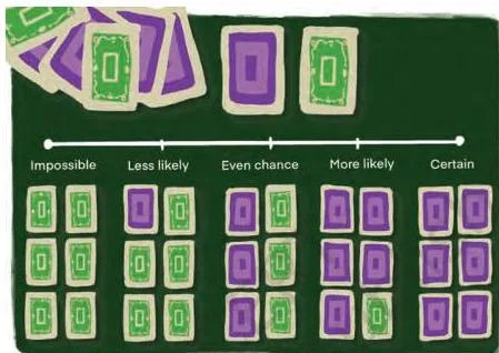
Before any formula, the chapter gives you a ruler. The probability scale runs from 0, meaning impossible, to 1, meaning certain, and every event in this chapter lands somewhere on it. The five scale labels the chapter uses are impossible, less likely, equally likely (even chance), more likely and certain.
A probability of 0.5 means even chance — just as likely to happen as not. A probability of 0.75 means 75%, which is more likely than not. Fractions, decimals and percentages are three ways of writing the same value.
The book’s purple-card deck shows the scale in action. With no purple cards in the deck, picking a purple card is impossible; add purple cards one by one and the probability slides from less likely to even chance to more likely; with all six cards purple, it is certain.
Fig 7.1 in the figure walkthrough below draws this scale as a line.
The book attaches one of five labels to everyday events so you can compare them without any arithmetic. Its own table of five events (Section 7.1.2):
| Event | Label | Why it carries that label |
|---|---|---|
| Getting a number greater than 6 on a die | Impossible | a die shows only 1 to 6 |
| Rolling a 3 on a standard die | Less likely | 3 is one face out of six |
| Flipping a coin and getting heads | Even chance | heads and tails are equally likely |
| Drawing any number from 2 to 10 from a deck of 52 cards | More likely | 36 of the 52 cards carry these numbers |
| Choosing a red sweet from a bag of all red sweets | Certain | every sweet is red |
Exercise Set 7.1 then asks you to rank four new events on this scale — from “the next Monday will come after Sunday” to “an elephant will walk through your classroom today” — and to give a reason for each label.
Experimental probability: counting what actually happened
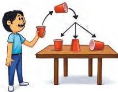
Some experiments give outcomes that are not equally likely — a tossed paper cup is the book’s example. When you cannot reason about fairness, you run the experiment and count what actually happens.
Experimental probability equals the number of times the event occurred divided by the total number of trials (Section 7.2.1). The book also calls this ratio the relative frequency of the event.
\[ \text{Experimental Probability} = \frac{\text{Number of times the event occurred}}{\text{Total number of trials}} \]
Worked example (original numbers): a die is rolled 30 times and lands on 6 exactly five times. The experimental probability of a 6 is \( \frac{5}{30} = \frac{1}{6} \approx 0.167 \), about 16.7%. Roll the same die 10 times and get two 6s, and the value is \( \frac{2}{10} = 0.2 \). Neither answer is wrong — small samples wobble.
The same counting works on data already collected, which is how Section 7.2.3 applies probability to statistics. Original example: a survey of 80 students finds 12 walk to school, so \( P(\text{walk}) = \frac{12}{80} = 0.15 \).
For a school of 1000 students, that gives an estimate of about \( 0.15 \times 1000 = 150 \) walkers. The estimate is only as good as the sample — the book’s sampling note says larger, more representative samples give surer estimates.
Exercise Set 7.2 makes this concrete with two do-it-yourself trials: toss a coin 20 times and record heads and tails, then toss a paper cup 100 times and record whether it lands on its bottom, top or side (Fig 7.5).
The cup matters because its three landing positions are not equally likely — that is exactly why the exercise assigns experimental probabilities instead of assuming one third each.
Theoretical probability: counting what is fair
When every outcome has the same chance — a fair die, a fair coin, a random draw — you can compute probability by counting, with no experiment needed. That is theoretical probability.
\[ P(A) = \frac{\text{Number of favourable outcomes}}{\text{Number of possible outcomes}} \]
\( P(A) \) is read as “the probability of event A”; the denominator is always the size of the sample space. The value always lies between 0 and 1, written \( 0 \leq P(A) \leq 1 \) (NCERT, Chapter Summary).
Worked example (original numbers): roll a fair die. What is the probability of an odd number? The favourable outcomes are 1, 3 and 5 — three of them — out of six possible outcomes, so \( P(\text{odd}) = \frac{3}{6} = \frac{1}{2} = 0.5 \).
Worked example (original numbers): pick a letter at random from the word MATHEMATICS. The word has 11 letters and M appears twice, so \( P(M) = \frac{2}{11} \approx 0.182 \). The book’s own example is the same idea with the word PROBABILITY — two Bs in 11 letters — and the repeated letter is exactly the point: it doubles the favourable count.
The fairness assumption is what makes the formula valid. The book’s Fair and Unbiased note explains that a fair coin is symmetrical, so heads and tails are equally likely, and a “random toss” means the coin falls freely. If the object is not symmetrical — the paper cup again — this formula has no right to be used.
The Law of Large Numbers and why the two probabilities differ
Here is the worry every student hits: “I rolled a die 12 times and got a 3 three times, so experimental P is \( \frac{3}{12} = 0.25 \), but theory says \( \frac{1}{6} \approx 0.167 \). Is something wrong?” No — and Exercise Set 7.2, question 6, asks exactly this.
Experimental probability comes from actual data and can sit anywhere near the theoretical value when trials are few. As the number of trials grows, it tends to close in on the theoretical value. That tendency is the Law of Large Numbers (Section 7.2.3).
Original worked example comparing the two: a die is rolled 30 times and shows 3 seven times. The experimental probability is \( \frac{7}{30} \approx 0.233 \); the theoretical probability is \( \frac{1}{6} \approx 0.167 \).
The gap is just small-sample wobble. Roll 600 times and you expect roughly 100 threes, so the experimental fraction settles near \( \frac{100}{600} \approx 0.167 \) — the two converge. The book’s Think and Reflect prompt sums it up: probability does not tell you what will happen next; it predicts what happens in the long run.
Here is the experimental-versus-theoretical comparison at a glance:
| Feature | Experimental probability | Theoretical probability |
|---|---|---|
| Data needed | actual trials or past records | none — reasoning only |
| Fairness assumption | none required — you count what happened | all outcomes equally likely |
| Formula | \( \frac{\text{occurred}}{\text{trials}} \) — also called relative frequency | \( \frac{\text{favourable}}{\text{possible}} \) |
| After many trials | tends toward the theoretical value — Law of Large Numbers | remains fixed |
Keep this table in mind whenever an exercise gives you a trial record and asks for a probability: decide first which column you are in.
Sample space, sample size and events
You cannot count favourable outcomes until you have the complete list to count from. That list is the sample space.
The sample space S is the set of all possible outcomes of a random experiment, with each outcome listed exactly once (Section 7.3.1). The number of outcomes is the sample size, written \( n(S) \).
- Rain tomorrow: \( S = \{\text{Rain, No Rain}\} \), so \( n(S) = 2 \)
- A match: \( S = \{\text{Win, Lose, Draw}\} \), so \( n(S) = 3 \)
- One coin: \( S = \{\text{H, T}\} \)
- One die: \( S = \{1, 2, 3, 4, 5, 6\} \)
- Two coins: \( S = \{\text{HH, HT, TH, TT}\} \), so \( n(S) = 4 \)
HT and TH are different outcomes because the two coins are separate objects: “heads on the first coin, tails on the second” is not the same toss as “tails on the first, heads on the second”. The book’s two-coin table lists all four in exactly this order.
An event is any one outcome or group of outcomes — a subset of the sample space (Section 7.3.2). The book’s examples: “at least one head” from two coins is \( E = \{\text{HH, HT, TH}\} \); “a number greater than 4” on a die is \( E = \{5, 6\} \).
Worked example (original numbers): toss a coin and roll a die together. The sample space has 12 outcomes: H1, H2, H3, H4, H5, H6, T1, T2, T3, T4, T5, T6. The event “a head with an odd number” contains H1, H3 and H5 — three favourable outcomes. So \( P = \frac{3}{12} = \frac{1}{4} = 0.25 \).
The book’s Think and Reflect prompt adds the detail rule: a sample space must be detailed enough for the question. {Rain, No Rain} is fine for “will it rain?”, but {No Rain, Drizzle, Light Rain, Heavy Rain} is needed once amounts of rain matter.
Tree diagrams for multi-step experiments
A multi-step experiment — toss a coin twice, roll a die three times — has outcomes made of several parts. A tree diagram lists every combination without missing one.
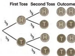
The book’s example is tossing a fair coin twice (Fig 7.6). The first toss branches into H and T; each branch splits again into H and T. The four paths are HH, HT, TH and TT — exactly the sample space — and each path is one of four equally likely outcomes.
So \( P(\text{HH}) = \frac{1}{4} = 0.25 \), matching the theoretical formula. Now the book’s Think and Reflect question: what is the probability of one head and one tail? That event collects two paths, HT and TH, so it is \( \frac{2}{4} = \frac{1}{2} \) — not \( \frac{1}{4} \).
The classic trap is the near-identical question “at least one head”. That event collects three paths — HH, HT, TH — so its probability is \( \frac{3}{4} \). Read the question carefully: “at least one” allows two heads; “exactly one” does not.
Exercise Set 7.4 asks you to draw trees for two fruit baskets and for pen colours. The starred end-of-chapter questions extend trees to draws without replacement, where the second branch changes after the first draw.
Formulas used in this chapter
Two formulas do the whole chapter, and both are printed in the book’s own summary. Use the table below as the revision snapshot — symbols on the left, meaning and use on the right.
| Formula | What the parts mean | When it applies |
|---|---|---|
| \( \text{Experimental Probability} = \frac{\text{Number of times the event occurred}}{\text{Total number of trials}} \) | numerator — how often the event happened; denominator — how many trials you ran; the result is also called relative frequency | data exists: trials you ran or records you collected; outcomes need not be equally likely |
| \( P(A) = \frac{\text{Number of favourable outcomes}}{\text{Number of possible outcomes}} \) | A is the event; favourable — outcomes that make A true; possible — all outcomes in the sample space | every outcome equally likely: fair coin, fair die, random draw |
Every probability these formulas produce sits between 0 and 1 — 0 impossible, 1 certain, most events in between. If your fraction ever comes out above 1, you have swapped numerator and denominator; re-read the question.
Figures in the chapter and how to read them
The diagrams below are the ones this chapter teaches from, each with its NCERT caption and a reading guide. If you are away from the PDF, these are the pictures the exercises depend on.
Read this figure as a number line for chance. The left end is 0 — impossible; the right end is 1 — certain. The book slides the purple-card position along the line: no purple cards at all puts it at 0, all six purple puts it at 1, and mixes in between sit at less likely, even chance or more likely.
Any event you label in Exercise Set 7.1 can be placed on this same line.
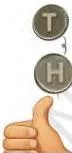
This pair of faces is the chapter’s first sample space: {H, T}, size 2. Because the coin is symmetrical, a fair toss gives each face probability \( \frac{1}{2} \) — the Fair and Unbiased note says the same thing.
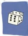
The die gives the sample space {1, 2, 3, 4, 5, 6}, size 6. Every face is equally likely, so any single number has probability \( \frac{1}{6} \approx 0.167 \) — the value that keeps coming back in examples, exercises and the Gambler’s Fallacy box.
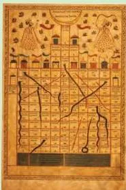
This cloth board is a Jñān-Chaupad game from 19th-century India — the ancestor of Snakes and Ladders, played with dice. The book includes it to connect dice and randomness to ancient games, and the Gambler’s Fallacy box returns to dice in Snakes and Ladders. The point for probability: dice games run on equally likely outcomes.
The cup is the chapter’s most important counter-example. It has three landing positions, but they are not equally likely — the cup is not symmetrical, so its centre of mass favours some positions. That is why Exercise Set 7.2 asks you to toss a cup 100 times and assign experimental probabilities instead of assuming one third each.
Read the tree from left to right. The first toss branches into H and T; each of those branches splits into H and T for the second toss. The four paths — HH, HT, TH, TT — are the sample space.
Count paths to get probabilities: one path (HH) is \( \frac{1}{4} \), two paths (HT, TH) are \( \frac{2}{4} = \frac{1}{2} \), three paths (HH, HT, TH) are \( \frac{3}{4} \).
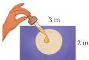
Question 16 is the chapter’s area-based probability, and it is an edge case: the probability is a ratio of areas, not a ratio of counts. A dye is dropped at random on the rectangle, and you want the chance it lands inside the circle of diameter 1 m. So \( P = \frac{\text{area of the circle}}{\text{area of the rectangle}} \).
The circle’s area is \( \pi \times (0.5)^2 \approx 0.785 \ \text{m}^2 \); read the rectangle’s length and breadth from the figure in the PDF, multiply them for its area, and divide.
Definitions you need to remember
The chapter builds a fixed vocabulary, and the starred exercises assume you know all of it. Each term below is one line: the name, the book’s meaning, nothing extra.
| Term | Meaning in one line |
|---|---|
| Probability | a measurement of how likely an event is, on a scale from 0 to 1 |
| Random experiment (random observation) | a repeatable action whose result cannot be predicted in advance, like tossing a coin |
| Outcome | one possible result of an experiment |
| Sample space | the set S of all possible outcomes, each listed exactly once |
| Sample size | \( n(S) \), the number of outcomes in the sample space |
| Event | a subset of the sample space: one outcome or a group of outcomes |
| Experimental probability | number of times the event occurred divided by the total number of trials |
| Relative frequency | the same ratio as experimental probability, seen as a frequency from actual data |
| Theoretical probability | favourable outcomes over possible outcomes, assuming all outcomes are equally likely |
| Fair (unbiased) | an object such as a symmetrical coin with no reason to favour one side |
| Population | the entire group you want to draw conclusions about, e.g. all students in a school |
| Sample | the part of the population you actually collect data from |
| Law of Large Numbers | experimental probability approaches theoretical probability as trials increase |
| Gambler’s Fallacy | the false belief that a run of past outcomes makes the opposite outcome more likely next; the coin or die has no memory |
Common mistakes in probability (and how to avoid them)
The errors below are the ones this chapter’s own exercises and Think and Reflect prompts warn about. Read each row twice: the mistake first, then the rule that stops it.
| Mistake | Correct rule | How to check your answer |
|---|---|---|
| Gambler’s Fallacy — believing three 6s make a 6 less likely next | each roll is independent; the die has no memory, so \( P(6) = \frac{1}{6} \) on every roll | ask yourself: can the die remember its last roll? No — so the next probability is unchanged |
| Expecting experimental and theoretical probabilities to match exactly | Exercise Set 7.2 Q6 exists for this: small trials differ, and the Law of Large Numbers closes the gap | compare occurred over trials with favourable over possible; a gap at small n is normal, not an error |
| Writing a sample space that misses an outcome or repeats one | a sample space must list every possible outcome once; the two-coin space is {HH, HT, TH, TT} | does every path on your tree appear once? Does \( n(S) \) equal the number of paths? |
| Confusing “at least one head” with “exactly one head” | at least one = {HH, HT, TH}, so \( \frac{3}{4} \); exactly one = {HT, TH}, so \( \frac{2}{4} = \frac{1}{2} \) | re-read the question: does it allow two heads? |
| Assuming a paper cup’s three landing positions are equally likely | the cup is not symmetrical, so it has no \( \frac{1}{3} \) each — use experimental probability | is there any physical reason one landing is favoured? If yes, do not use the theoretical formula |
| Counting only one B in PROBABILITY (repeated letters) | PROBABILITY has two Bs and MATHEMATICS has two Ms — favourable counts every occurrence, not distinct letters | list the letters and tick each occurrence of the target letter |
| Writing a probability above 1, or a percentage above 100% | the scale runs 0 to 1; favourable can never exceed possible | if your fraction is greater than 1, you swapped numerator and denominator |
How to use this chapter for exam preparation
By the end of the chapter you should be able to do six things. These six skills are exactly what the exercises in the book ask for.
- Rank events on the 0 to 1 probability scale with a label and a reason
- Compute an experimental probability from a frequency table or a trial record
- Compute a theoretical probability by counting favourable and possible outcomes
- Write a sample space and its size \( n(S) \)
- Draw and read a tree diagram for a multi-step experiment
- Estimate a population value from a sample using its relative frequency
For any probability question, the same three-step attack works:
- Identify the experiment and write the full sample space — every outcome once.
- Count the favourable outcomes for the event the question names.
- Write favourable over possible (theoretical) or occurred over trials (experimental), then check the result sits between 0 and 1.
The end-of-chapter exercises test these skills in a clear order. Use the map below to pick your practice.
| End-of-chapter questions | What they test |
|---|---|
| 1–2 | vocabulary (impossible, sample space, certain) and relative frequency |
| 3 | judging when outcomes are equally likely |
| 4 | writing sample spaces and basic probability — two coins, numbered cards, a die, balls |
| 5–6 | simple counting and arranging combinations in a table |
| 7 | reading probabilities from a frequency table (tyre distances) |
| 8 | letter cards, including the “not an E” case |
| 9–12 | starred — a spinner (Fig 7.7 in the PDF), dice, draws without replacement, multi-step counting |
| 13–15 | constructing and judging sample spaces |
| 16 | area-based probability with Fig 7.8 |
The starred questions are harder but use the same three steps. Question 16’s area ratio is the one unusual case — see the Fig 7.8 reading above.
One reminder: textbook contents and the examinable syllabus are not always identical. Check the current official syllabus on the CBSE website before deciding what to revise.
Key takeaways from Chapter 7
Six or seven bullets is enough to revise the night before. Each bullet below condenses the chapter’s own summary.
- Probability is a measurement of how likely an event is, on a scale from 0 (impossible) to 1 (certain); the probability of an event A is written \( P(A) \), with \( 0 \leq P(A) \leq 1 \).
- Experimental probability is the number of times the event occurred divided by the total number of trials — also called relative frequency.
- Theoretical probability assumes equally likely outcomes: \( P(A) = \frac{\text{favourable}}{\text{possible}} \).
- The sample space S lists every possible outcome exactly once; \( n(S) \) is its size.
- An event is a subset of the sample space.
- Tree diagrams list and visualise all outcomes of a multi-step experiment, and their paths give probabilities by counting.
- With enough trials, experimental probability approaches theoretical probability — the Law of Large Numbers.
Related NCERT Class 9 resources
This listing is maintained for the 2026-27 academic session using the NCERT textbook information available to us. NCERT remains the authority for confirming the latest edition.
- The NCERT Class 9 Mathematics book page lists every chapter of Ganita Manjari, including this one.
- The Class 9 hub gathers the NCERT textbooks and notes for all Class 9 subjects.
- Chapter 6, Measuring Space: Perimeter and Area, is the chapter that comes just before probability in this book.
- Chapter 8, Predicting What Comes Next: Exploring Sequences and Progressions, follows right after.
Sources and data verification
- The contents, figures and exercises described on this page come from the NCERT Class 9 Mathematics textbook (Ganita Manjari, Part I), Chapter 7, The Mathematics of Maybe: Introduction to Probability, as published on ncert.nic.in.
- This page covers that single chapter and no other book or edition.
- It is maintained for the current academic session using the NCERT information available to us.
- NCERT settles textbooks, editions and official PDFs; CBSE settles the curriculum, syllabus and examinations.
Reference: NCERT Class 9 Mathematics textbook, chapter 7, official edition on ncert.nic.in.
Frequently asked questions
What is the difference between experimental and theoretical probability in Class 9 Maths Chapter 7?
Experimental probability comes from actual data — the number of times the event occurred divided by the total number of trials — and the book also calls it relative frequency. Theoretical probability assumes all outcomes are equally likely and uses favourable outcomes over possible outcomes, with no experiment needed.
With few trials the two can differ; the Law of Large Numbers says they get closer as trials increase.
Does rolling three sixes in a row make a six less likely on the next roll?
No. The Gambler’s Fallacy box exists for exactly this belief. Each roll of a fair die is independent — the die has no memory — so the probability of a 6 is \( \frac{1}{6} \approx 0.167 \) on every roll, including right after three sixes.
Why is the probability scale from 0 to 1, and what does a probability of 0.75 mean?
Zero means impossible and 1 means certain, so the scale from 0 to 1 covers every possible likelihood. A probability of 0.75 is the same as 75% — since it is above 0.5, the event is more likely than not.
What is the sample space when two coins are tossed, and why are HT and TH different outcomes?
The sample space is \( S = \{\text{HH, HT, TH, TT}\} \), so \( n(S) = 4 \). HT and TH are different because the two coins are separate objects: HT means heads on the first coin and tails on the second, while TH is the reverse. This distinction matters for events like “exactly one head”, which has probability \( \frac{2}{4} = \frac{1}{2} \).
How do you estimate the number of students in a school who prefer a club when only a sample is surveyed?
Use the sample fraction as the experimental probability and scale it to the school. If 14 of 50 sampled students prefer the chess club, the estimate for a school of 750 students is \( \frac{14}{50} \times 750 = 210 \) students. The book’s sampling note adds that larger, more representative samples make the estimate more reliable.
Why did my experimental probability for heads not come out to exactly 1/2?
Because a small number of tosses is a small sample. In 20 tosses you might get 12 heads, giving \( \frac{12}{20} = 0.6 \), or 8 heads, giving 0.4 — both are normal. The Law of Large Numbers says the experimental fraction settles toward \( \frac{1}{2} \) as the number of tosses grows.
Reference: NCERT Class 9 Mathematics textbook, chapter 7, official edition on ncert.nic.in.
Explore Class 9 Mathematics Books
- Previous: Measuring Space: Perimeter and Area
- Next: Predicting What Comes Next: Exploring Sequences and Progressions
Related chapters:
- Orienting Yourself: The Use of Coordinates
- Introduction to Linear Polynomials
- The World of Numbers